Introduction
Hair loss is a significant problem in now a days. Even people in younger age groups are going through remarkable hair loss problems. Most common reasons are stress, poor diet, inadequate sleep, male pattern baldness etc.
Conventionally, for determining the stage of hair loss, one would need to go to a clinic. At HKVitals, we aim to change the conventional methods. The idea is to make hair test accessible to people at home, with a simple hair scan by phone camera.
Let’s dive into different approaches and algorithms we used for achieving this!
Ground Building – Starting up with Image Processing
During the initial phase of development, I tried achieving hair fall stage detection using Artificial Intelligence, however due to lack of proper datasets I had to fall back to Image Processing using OpenCV, idea was to use image processing, start collecting the data and once significant data is there, train the model using CNN and reinforce it as we collect more data.
First Approach – Pattern Matching by Mean Square Error
The first approach we opted for was Image Processing. We had primarily two reasons to choose Computer Vision. First, we were operating with images and computer vision based image processing is natural inclination. Second, the Mean Square Error approach can be readily implemented using Image Processing libraries like OpenCV.
Let’s understand how a simple mean squared error method can provide us the results we need. There are a few globally accepted hair loss scales, one of which is Norwood-Hamilton scale. This scale is only for males. For females, we chose Savin scale. Both of these scales focus on the top head view. In females, hair loss starts from the scalp.
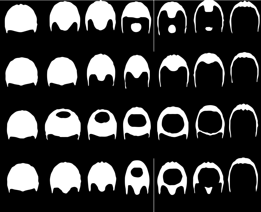
Norwood Hamilton Scale
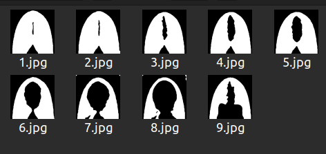
Savin Scale
In the Norwood Hamilton scale, each column represents a stage. Each stage has 4 variants. Starting from left, first column represents all four variants of stage 1, the second column represents all four variants of stage 2 and so on.
In the Savin scale, each image represents a stage. 1.jpg represents stage 1, 2.jpg represents stage 2 and so on. The ninth stage in Savin scale is known as Frontal hair loss.
If you notice, all these images do not look normal. It’s because they underwent binarization. To binarize an image is to convert it in a format where all its pixels are restricted to either of the two colors, as specified during the process. The most common binarization technique is to choose black and white combination for color choices. The black area surrounded by white portions represents loss of hair in the above images.
Also, the black areas beyond the white portion represents background, which we tend to ignore. The concept is to compare the user’s image with all these binarized images. The closest resembling threshold pattern to the user’s image is supposed to be the user’s hair pattern, after which we simply check which column that binarized image belongs to. For example, if it lies in the third column then the user’s hair is indeed in stage 3.
Using OpenCV, we performed appropriate threshold of images by OTSU algorithm. We chose OTSU because it is impossible to decide a static set of pixel values for binarizing every image as the environmental factors are extremely dynamic. With different lighting conditions, binarization gets affected. OTSU & Triangle, both are well known methods for performing binarization when you are not sure what values will work in general or when you cannot generalise threshold values for all images.
Even so, we went with OTSU because Otsu’s method is an adaptive thresholding technique that automatically determines the optimal threshold value by maximizing the variance between two classes of pixels: foreground and background while the Triangle method is a non-parametric thresholding technique that computes the threshold as the point where a line connecting the histogram’s peak to the maximum intensity intersects with the histogram. For my use case, OTSU proved to be much better.
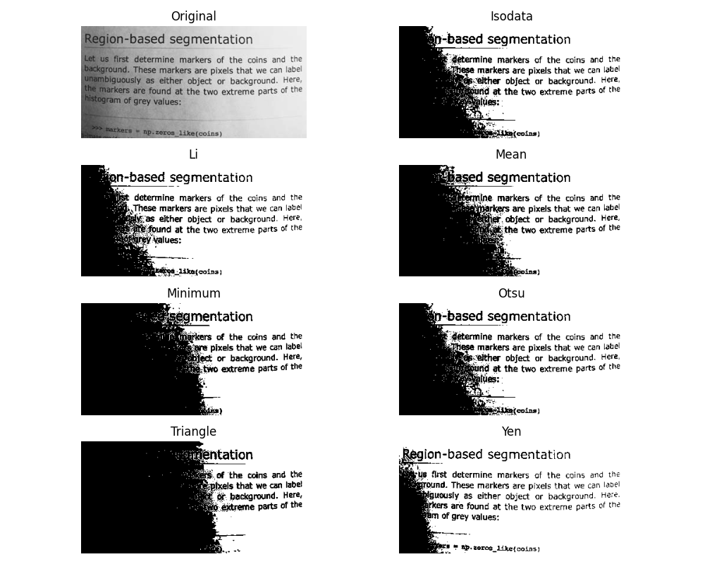
Source: Scikit
The threshold image had too much noise and didn’t look as smooth and clean as we needed for appropriate comparison. Also, minute details were very highlighted and we needed a way to eliminate little details since that affected thresholding significantly. In order to achieve this, I used iterative blur and clustering using KNN algorithm. Blurring followed by each KNN, first with K=4 and then with K=2.
Once done, we looped through each image in the Norwood Hamilton set and compared user’s image with it. The method of comparison used here is Mean Square Error. In each iteration, you subtract ith Norwood Hamilton image from the user’s threshold image to get the error. Then you square it using numpy.
Lastly, you get the mean by dividing the sum of error by the product of width and height of image. All that’s left is to match the error index to the respective image index and get the final prediction.
We fetched three most possible stages using the MSE algorithm and we called it prediction array. Normally, the stage corresponding to the 0th index should be the correctly predicted stage since it has the least error as compared to others in the array. However, interestingly, after close observation it was concluded that in most cases the stage at 1st index is the correct one. That’s how we built this.
Challenges in this approach – Glare Problem
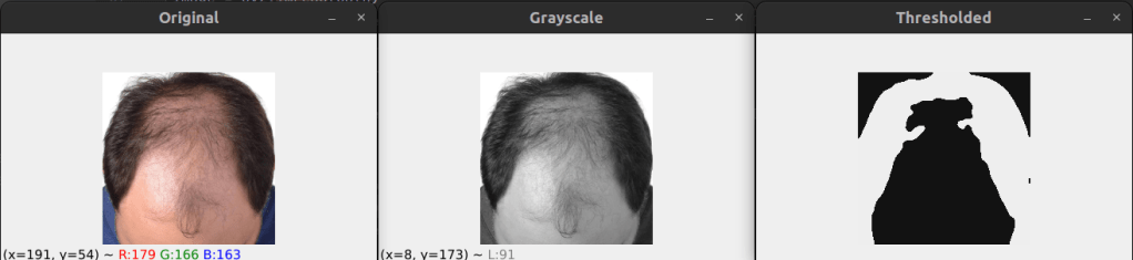
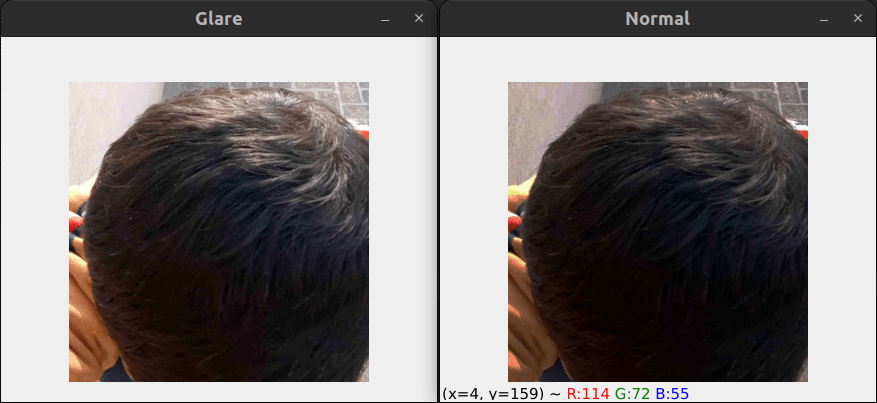
The results were near perfection with no accuracy issues but as we deployed this tech for testing in the private beta, we were introduced to the haunting glare problem. In case of uneven lighting or glare in the image, the threshold image gets severely affected. Due to this, the comparison between the user’s image and Norwood model images becomes absurd and started giving higher stage of hair fall as a false result. We tried glare area detection to some extent and image in-painting. That did not work either.
For example, in the below image, presence of glare is affecting the binarization of image and hence the final comparable image, Outcome of the model from glare image (Left side image) is stage 3, however when it is passed with image without glare (Right side Image) it is giving correct result as stage 1.
Glare problem !! Ah Interesting one … Lets solve this
This approach is an enhancement over the first approach. In this approach, I used a polynomial function instead of a linear one for gamma correction and contrast enhancement. The reason for using a polynomial function is the fact that we don’t want to drive all pixel values up or down by extremely high or extremely low factors. We only want small changes that normalize the image overall.
There are two variants of this approach, RG ( Reduce Glare ) & RGEC ( Reduce Glare & Enhance Contrast ). The RG variant only does gamma correction alternatively while the RGEC variant does gamma correction and then improves the contrast.
Before every gamma correction, we adjusted the pixels using two polynomial functions. One of the polynomial functions looked something like:
1.657766 X - 0.009157128 X2 + 0.00002579473 X3If you’re wondering how I arrived at such a random equation, it’s because it’s not exactly random. This is mathematics. Higher-degree polynomials (like cubic polynomials) are used because they can capture non-linear relationships in intensity mappings better than linear transformations.
Also, suppose I want to correct an image that is slightly overexposed, collecting pixel intensity mappings from a reference well-exposed image or manually defining how certain intensities should be adjusted does help in getting pixel intensity points. I then used these points to fit a polynomial curve.
Even so, it wasn’t as perfect as we imagined. I made slight coefficient adjustments on my own with close observation over images processed through my polynomial functions.
This approach worked very well on most lighting conditions.
Challenges in this approach – Inconsistent Results
Images reproduced by RGEC gave better results when passed by the OTSU layer but in some normal cases it produced results worse than the Mean Square Error approach. Even though this was an extraordinary improvement in the computer vision world, we decided not to deploy this on production due to the absurd results on normal lighting condition images sometimes.
Lets try something else to solve the Glaring !! .. How about composite Algorithm
The third approach focuses on utilizing multiple techniques to our favor. We call it Composite Algorithm. We decided to keep the gamma correction part from the second approach and use three different algorithms for determining the stage of hair loss.
The three algorithms used were – Mean Square Error, SSIM & Histogram Similarity. We already talked about the Mean Square Error approach, SSIM stands for Structure Similarity Index Measure. It is a part of skimage library and it’s used for finding similarity between two images. Histogram similarity is a traditional method used for comparing the pixel intensity graphs between images. Based on these three methods, we prepared a score as follows:
Composite Score = 0.5 * df.hist_score + 0.3 * df.ssim_score + 0.2 / df.mse_score
Based on this score, we made a prediction of hair loss stages of the user’s image.
Challenges in this approach – Low/Same Accuracy
This approach worked just like the polynomial function approach, slightly better at times. However, the results were still not satisfactory. We were playing at around 60 % worst case accuracy and around 70 % average accuracy. The average accuracy was almost the same as achieved through Polynomial Functions. This is where computer vision peaked. Even though accuracy was low, we decided to release it for limited audience and started gathering data. Once we realized that we have enough data from audience, we decided to prepare data and use this for training CNN Model.
We have enough data now .. Lets train our CNN model
We did not start with CNN/DNN based model since we had no data for any kind of training back then. Though, at this point we had sufficient hair data for males. We did not know how exactly the chosen model will react to glare images but I knew it would have intelligence, unlike the traditional computer vision techniques. Also, the threshold techniques are very sensitive to glare since their core functionality works on pixel intensities, which is not the case with AI models.
This time we went for a classification model and we chose YOLOv8 for this task. Transfer learning has cured the hunger for large datasets. YOLO has been doing good with accuracy of smaller models as well.
After augmenting the originally available data, we had sufficient images for all stages corresponding to hair loss in males. We used the small variant of YOLOv8 for training the model.
Challenges in this approach – Unseen Patterns, Limited Data & Errors in Classification
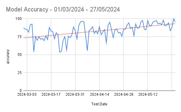
This approach has proved to be the best until now. We are now playing around 80 % worst case accuracy and around 95 % average accuracy, peaking close to 100 % on some days. However, we still need female hair loss dataset for training a classifier for females. The challenge is to accumulate sufficient data for all stages of female hair loss.
Apart from this, this approach tends to face problems in case of outlier cases. Some hair patterns are just odd while some are rare. Unseen patterns & erroneous classifications need to be augmented and re-trained over a fixed interval in order to get the best results in the long run.
YOLOv8 and similar deep learning models are trained on large datasets that include a variety of real-world conditions, including images with glare, reflections, shadows, and other imperfections. This extensive training helps the model learn to generalise and recognise patterns despite these variations. Deep learning models automatically learn relevant features directly from the data. They can extract complex patterns and high-level abstractions that make them robust to noise and distortions such as glare.
Usability Challenges
We were sorted with our approaches towards the problem we were eagerly trying to solve. However, when we deployed this technology in the initial testing phase, we were introduced to real world challenges we did not comprehend earlier. How user can take picture of his head without looking at the screen, the idea of auto head detection popped in & we created a model for auto head detection and clicking the picture automatically as soon as head is detected. This sounds simple, but it wasn’t really. Let’s see how we overcome different roadblocks here.
Challenge 1 – Compatibility Issues – Flutter and TensorFlow
We were on our way implementing auto head detection along with auto head cropping post detection in our mobile app, which apparently had tons of compatibility issues. The compatibility issues came into play when we tried integrating custom trained TensorFlow model for head detection in Flutter. Flutter wasn’t ready for TensorFlow & TensorFlow wasn’t ready for Flutter. There was no direct way for integration of TensorFlow models in Flutter.
Solution
We decided to do it the twisted way. We played this frame-wise. As soon as head was detected, we sent the detected camera frame to native app sides where further processing was done using that image frame. We were still training different kinds of models for a smoother head detection in order to reduce latency between image capture and image sending activities. We later switched to Vertex AI Edge model and faced negligible compatibility issues. The methods of integration ensured zero latency!
Challenge 2 – Partial Head Detection
Another significant challenge we faced during early the testing phase was partial head detection. For instance, have a look at this:

As soon as the model saw a frame with a human head, it didn’t matter if it was a full or partial head, the image was captured.
Solution
We re-trained the model with a few key changes this time. We cleaned my training data off any images that contained partial heads. We rather included them as negative samples. This significantly solved the problem.
Challenge 3 – Face Features Detection
I was chasing solutions and problems were chasing me. I was looping between both and so was my mind. The next challenge was way too major to ignore. We were facing weird false detection by the model. Model was great at this point, at least to our knowledge. But when we rolled out this technology for testing, many people faced absurd results due to false detection, which brought heat to this challenge. For instance:
False Detection Type 1 – Forehead Detection
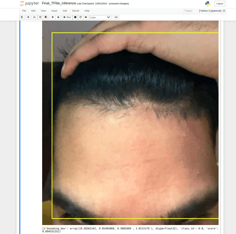
Our ML model detects forehead as well as hand along with hair. We do not want that. In fact, we want our model to reject this image as this is not top head.
Solution
With the public face datasets available over the internet, we resized all images in the dataset to a fixed resolution, then cropped from a specific point on Y-axis in order to obtain only the upper half face images. This data was served to the model as negative samples and retraining fixed the issue to a huge extent. This mostly eliminated the forehead detection problem. However, the “hand on top of head” problem couldn’t be solved by this method due to lack of appropriate datasets for this. We solved this problem by using a hand detection model.
False Detection Type 2 – Face Detection

Our ML model detects hair successfully but the bounding boxes were not accurate enough. Several times the model detected eyebrows and forehead along with top head. This created problems with KNN and threshold algorithm. This issue was almost guaranteed to emerge if the image was captured when the user was looking into the camera while testing their hair. Also, a few times our model falsely detected human faces as top heads.
Solution
The root cause of this issue lies in the detection of hair even when face is visible in camera frame. The facial features made the algorithm prone to clustering and threshold errors. The simplest idea to eliminate this error was to remove the face factor from our detection somehow. We achieved this by using ML Kit for anti face detection. In case head and face were present in the camera frame at the same time, that particular frame was rejected. The detection process would only move forward when the top head is visible and not the face. This solved the face detection problem. However, to make our custom trained model even more robust, we added faces as negative samples.
Conclusion
Working with computer vision algorithms, we were able to achieve good average accuracy in terms of daily classification. Honestly, it has been a steady research & development since the beginning and the technical aspects used serve as an epitome for the computer vision community. Artificial Intelligence surpassed Computer Vision in terms of accuracy and robustness because of the way it learns from data. Though we strongly believe Computer Vision has a whole lot of impressive stuff coming up in the future.
We are open to any suggestions and ideas that you believe we should know or implement. Please let us know in the comments.
Go ahead and download the HKVitals app for a highly accurate hair test!
Download the HKVitals app here
4 Easy Steps To Know Your Hair fall Stage
Step 1
Tap on “Profile”

Step 2
Tap on “HairScanr”

Step 3
Select your Gender & Tap on “Get Started”

Step 4
Check your Hair Test Result

The above outcome is a based on our experience while solving this problem, your experience might be different here and we are excited to hear your feedback and suggestions for the same. Please feel free to drop a comment, would love to have a chat on the same.
